LaTex 系列 - 4. TikZ 绘图

LaTex 中为了展示一个图片，需要使用 \includegraphics 命令，具体做法如下： - 编写 matlab/python 代码绘制曲线 - 保存图片为 pdf 格式，按照LaTex文档要求放置到指定路径 - 在 LaTex 文档中使用 \includegraphics 命令引入图片

这种方式可以在 LaTex 文档中展示图片，但是需要注意的是，图片的大小和位置需要手动调整，否则会影响文档的布局。

这里介绍一个便捷的工具 – TikZ

下面通过几个例子展示如何使用 TikZ 绘图。

例 1

\begin{tikzpicture}[>=stealth, scale=1]
  % 开始 tikzpicture 环境。
  % 选项：
  %   >=stealth  表示之后所有的箭头 (->) 默认使用 “stealth” 箭头样式；
  %   scale=1    图形整体缩放比例为 1（即不缩放）。

  % 坐标轴
  \draw[->] (0,0) -- (5,0) node[below] {$t$};
  % 画横轴：
  %   从坐标 (0,0) 画到 (5,0)，并在终点加一个箭头（因为使用了 ->）。
  %   在终点 (5,0) 上附着一个 node，位置在 below（线段下方），内容为 t，
  %   作为横轴标签。

  \draw[->] (0,-2.2) -- (0,2.8) node[left] {$x(t)$};
  % 画纵轴：
  %   从 (0,-2.2) 画到 (0,2.8)，在顶部加箭头。
  %   在终点处加一个 node，位置在 left（线段左侧），内容为 x(t)，
  %   作为纵轴标签。

  \draw[dashed,gray] (0,0) -- (5,0);
  % 画一条灰色虚线：
  %   从 (0,0) 到 (5,0)，与横轴重合，用来表示 x(t)=0 这条“零线”。

  % 用公式 x(t) = 2.4 e^{-t} 画一条轨迹
  \draw[thick,blue, domain=0:5, samples=100]
    plot (\x,{2.4*exp(-\x)});
  % 画第一条曲线：
  %   线条样式：
  %     thick  加粗；
  %     blue   蓝色；
  %     domain=0:5   自变量 \x 的取值范围是 0 到 5；
  %     samples=100  在区间 [0,5] 上取 100 个采样点来近似这条曲线。
  %   plot (\x,{2.4*exp(-\x)})：
  %     TikZ 自动把 \x 当作横坐标变量；
  %     纵坐标是 {2.4*exp(-\x)}，即 y = 2.4 * e^{-x}；
  %     所以这条曲线表示解轨迹 x(t) = 2.4 e^{-t}。

  % 再画一条 x(t) = -1.6 e^{-t} 的轨迹
  \draw[thick,blue, domain=0:5, samples=100]
    plot (\x,{-1.6*exp(-\x)});
  % 第二条曲线：
  %   样式同上（加粗、蓝色、[0,5] 区间、100 个采样点）。
  %   纵坐标公式为 -1.6*exp(-\x)，即 y = -1.6 e^{-x}，
  %   表示从负初值 -1.6 出发，同样指数衰减到 0 的解轨迹。

\end{tikzpicture}

运行效果

例 2

\begin{tikzpicture}[>=stealth, scale=1]
  % 开始 tikzpicture 环境，用来绘图。
  % 选项：
  %   >=stealth ：把之后所有 "->" 箭头的箭头样式设为 stealth；
  %   scale=1   ：整体缩放因子为 1（不缩放，如果改成 1.2 就会整体放大 1.2 倍）。

  % 坐标轴
  \draw[->] (0,0) -- (5,0) node[below] {$t$};
  % 画横轴：
  %   从点 (0,0) 到 (5,0) 画一条直线，末端带箭头（因为使用了 "->"）。
  %   在终点 (5,0) 上附着一个 node，位置在 below（线段下方），内容为 t，
  %   作为横轴的标签。

  \draw[->] (0,-2.2) -- (0,2.8) node[left] {$x(t)$};
  % 画纵轴：
  %   从 (0,-2.2) 到 (0,2.8) 画一条直线，末端带箭头。
  %   在终点左侧放置一个 node，内容为 x(t)，作为纵轴标签。

  \draw[dashed,gray] (0,0) -- (5,0);
  % 画一条灰色虚线：
  %   从 (0,0) 到 (5,0)，与横轴重合；
  %   样式为 dashed（虚线）、gray（灰色），表示 x(t)=0 的零线。

  % 在 t=0 左侧标注不同的初值
  \draw (0,2.4) node[left] {$x_0^{(1)}$};
  % 在坐标 (0,2.4) 放一个 node，位置在该点左侧（left），
  % 文本为 x_0^{(1)}，表示第一条轨迹的初始值。

  \draw (0,1.5) node[left] {$x_0^{(2)}$};
  % 在 (0,1.5) 左侧标注 x_0^{(2)}。

  \draw (0,0.7) node[left] {$x_0^{(3)}$};
  % 在 (0,0.7) 左侧标注 x_0^{(3)}。

  \draw (0,-0.8) node[left] {$x_0^{(4)}$};
  % 在 (0,-0.8) 左侧标注 x_0^{(4)}。

  \draw (0,-1.6) node[left] {$x_0^{(5)}$};
  % 在 (0,-1.6) 左侧标注 x_0^{(5)}。
  % 这五个标记一起表示：在 t=0 时，系统可能的五个不同初始状态 x_0^{(i)}。

  % 用 x(t) = x0 * e^{-t} 画 5 条轨迹
  \foreach \xzero in {2.4, 1.5, 0.7, -0.8, -1.6} {
    % \foreach 是 TikZ 的循环语句：
    %   循环变量 \xzero 依次取 2.4, 1.5, 0.7, -0.8, -1.6 这五个值。
    %   对每个 \xzero，都执行大括号中的 \draw 命令，画出一条对应初值的轨迹。

    \draw[thick,blue, domain=0:5, samples=100]
      plot (\x,{\xzero*exp(-\x)});
    % 对当前的初值 x0=\xzero 画出解轨迹 x(t)=x0*e^{-t}：
    %   thick     ：线条加粗；
    %   blue      ：线条颜色为蓝色；
    %   domain=0:5：自变量 \x 的范围是 [0,5]；
    %   samples=100：在这个区间内取 100 个采样点来近似这条曲线。
    %   plot (\x,{...})：
    %     横坐标为 \x，纵坐标为 \xzero*exp(-\x)，
    %     即从不同 x0 出发的指数衰减轨迹。
  }

  % \node at (2.6,2.4) {\small 好的 $F$};
  % \node at (2.5,-2) {任意 $x_0$ 都收敛到 0};
  % 上面两行被注释掉了（行首有 %，LaTeX 不会执行）：
  %   如果取消注释，它们会在指定坐标位置放置说明文字，
  %   用来说明这是一个“好的 F（反馈/映射）”，任意初值都收敛到 0。

\end{tikzpicture}
% 结束 tikzpicture 环境，整幅图形绘制完成。

运行效果

例 3

\begin{tikzpicture}
  % 开始一个 TikZ 图环境，pgfplots 的 axis 环境也放在 tikzpicture 里。

  \begin{axis}[
    % 开始 pgfplots 的坐标轴环境，用来自动生成坐标系和函数图像。
    axis lines=middle,
    % 让坐标轴穿过原点，并且只画两条“中间”的坐标轴（而不是四周的边框）。
    % 即 x 轴和 y 轴都从原点向两边延伸，看起来像数学课本上的坐标系。
    xlabel={$t$},
    % 设置横轴的标签（label），显示为数学模式的 t。
    ylabel={$x(t)$},
    % 设置纵轴的标签，显示为数学模式的 x(t)。
    xmin=0, xmax=6,
    % 设置 x 轴显示范围：从 0 到 5。
    % 图中不会画出超过这个范围之外的内容。
    ymin=-2.2, ymax=2.8,
    % 设置 y 轴显示范围：从 -2.2 到 2.8。
    % 方便把所有轨迹都放在同一视窗里。
  ]
    % 以上是 axis 环境的可选参数列表，方括号结束到这里。

    % x(t) = 2.4 e^{-t}
    \addplot[blue, thick, domain=0:5] {2.4*exp(-x)};
    % 使用 pgfplots 画第一条函数曲线：
    %   关键字 \addplot 表示“添加一条曲线”。
    %   [blue, thick, domain=0:5] 是画图选项：
    %       blue  曲线为蓝色；
    %       thick 线条加粗；
    %       domain=0:5 自变量 x 的取值范围是 0 到 5。
    %   花括号里的 {2.4*exp(-x)} 是函数表达式：
    %       变量名是 x（pgfplots 约定俗成）；
    %       表示 y = 2.4 * e^{-x}，即 x(t)=2.4 e^{-t} 这条指数衰减曲线。

    % x(t) = -1.6 e^{-t}
    \addplot[blue, thick, domain=0:5] {-1.6*exp(-x)};
    % 第二条函数曲线：
    %   同样是蓝色、加粗、定义域 0~5；
    %   函数为 y = -1.6 * e^{-x}，即从负初始值 -1.6 出发的衰减轨迹。
    %   两条曲线一起表示不同初始值的解，都随 t 增大而趋向 0。

  \end{axis}
  % 结束坐标轴环境，坐标系和里面画的函数到此为止。

\end{tikzpicture}
% 结束 tikzpicture 环境，这个图形块就画完了。

运行效果

例 4

\usetikzlibrary{arrows.meta,positioning,shapes.geometric}

\begin{tikzpicture}[
    % 开始TikZ图形环境，方括号内是全局样式设置    
    >=Stealth,
    % 设置默认箭头类型为Stealth（三角形尖头箭头）    
    box/.style={
        % 定义名为"box"的样式，用于两个蓝色方框        
        rectangle,
        % 形状为矩形        
        rounded corners=15pt,
        % 圆角半径为15pt，使矩形四角变圆        
        minimum width=5cm,
        % 最小宽度5厘米        
        minimum height=1.8cm,
        % 最小高度1.8厘米        
        fill=blue!60,
        % 填充颜色为60%蓝色（蓝色与白色混合60:40）        
        draw=blue!70,
        % 边框颜色为70%蓝色        
        line width=2pt,
        % 边框线宽2pt        
        text=white,
        % 文字颜色为白色        
        font=\Large\bfseries,
        % 字体为Large大小且加粗        
        align=center
        % 文字居中对齐
    },    
    title/.style={
        % 定义名为"title"的样式，用于红色标题框        
        rectangle,
        % 形状为矩形        
        minimum width=7cm,
        % 最小宽度7厘米        
        minimum height=1.2cm,
        % 最小高度1.2厘米        
        fill=red!80!black,
        % 填充颜色：80%红色+20%黑色，产生深红色        
        text=white,
        % 文字颜色为白色        
        font=\huge\bfseries
        % 字体为huge大小且加粗
    },    
    arrow/.style={
        % 定义名为"arrow"的样式，用于弧形箭头        
        line width=4pt,
        % 箭头线宽4pt        
        blue!70,
        % 箭头颜色为70%蓝色        
        ->,
        % 线条末端添加箭头        
        >=Stealth
        % 箭头样式为Stealth型
    }
]
% 样式定义结束

    % 标题
    \node[title] (title) at (0, 3.8) {Feedback Loop};
    % 创建一个节点：
    % [title]: 应用之前定义的title样式
    % (title): 给这个节点命名为title（虽然后面没用到这个名字）
    % at (0, 2.8): 位置在坐标(0, 2.8)，即x=0, y=2.8
    % {Feedback Loop}: 节点中显示的文字内容
    
    % 左侧方框
    \node[box] (action) at (-3.2, 0) {Action or Stimulus};
    % 创建左侧蓝色方框：
    % [box]: 应用box样式
    % (action): 节点命名为action，后面绘制箭头时会用到
    % at (-3.2, 0): 位置在x=-3.2, y=0（左侧）
    % {Action or Stimulus}: 显示的文字
    
    % 右侧方框
    \node[box] (response) at (3.2, 0) {Response (Feedback)};
    % 创建右侧蓝色方框：
    % [box]: 应用box样式
    % (response): 节点命名为response
    % at (3.2, 0): 位置在x=3.2, y=0（右侧）
    % {Response (Feedback)}: 显示的文字
    
    % 上方弧形箭头（从左到右）- 从标题下方经过
    \draw[arrow] (action.north) to[out=70, in=110] (response.north);
    % 绘制上方的弧形箭头：
    % [arrow]: 应用arrow样式
    % (action.north): 起点是action节点的北侧（上方中心点）
    % to[out=70, in=110]: 使用贝塞尔曲线连接
    %   out=70: 从起点以70度角度出发（0度是正右，90度是正上）
    %   in=110: 以110度角度进入终点
    % (response.north): 终点是response节点的北侧
    
    % 下方弧形箭头（从右到左）
    \draw[arrow] (response.south) to[out=-110, in=-70] (action.south);
    % 绘制下方的弧形箭头：
    % [arrow]: 应用arrow样式
    % (response.south): 起点是response节点的南侧（下方中心点）
    % to[out=-110, in=-70]: 使用贝塞尔曲线
    %   out=-110: 从起点以-110度（即向左下）出发
    %   in=-70: 以-70度（即从右下）进入终点
    % (action.south): 终点是action节点的南侧

\end{tikzpicture}

运行效果

例 5

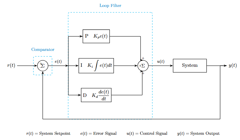
\usetikzlibrary{arrows.meta,positioning,calc,fit}
%\usepackage{mathptmx} % Times New Roman 字体

\begin{tikzpicture}[
    % 开始TikZ绘图环境，方括号内定义全局样式    
    >=Stealth,
    % 设置默认箭头样式为Stealth（三角形箭头）    
    thick,
    % 设置所有线条为粗线    
    % 定义各种节点样式
    block/.style={
        % 定义名为"block"的样式，用于绘制方框（如P、I、D、System）
        draw,
        % 绘制边框
        rectangle,
        % 形状为矩形        
        minimum height=1cm,
        % 最小高度1厘米        
        minimum width=2cm,
        % 最小宽度2厘米        
        align=center,
        % 文本居中对齐        
        line width=0.8pt
        % 边框线宽0.8pt
    },    
    sum/.style={
        % 定义名为"sum"的样式，用于绘制求和器（圆圈）        
        draw,
        % 绘制边框        
        circle,
        % 形状为圆形        
        inner sep=0pt,
        % 内部间距为0（文字紧贴边框）        
        minimum size=8mm,
        % 圆的最小直径8毫米        
        line width=0.8pt
        % 边框线宽0.8pt
    },    
    dashedbox/.style={
        % 定义名为"dashedbox"的样式，用于绘制虚线框        
        draw=cyan!60,
        % 边框颜色为60%青色        
        dashed,
        % 边框为虚线        
        line width=1pt,
        % 虚线线宽1pt        
        rounded corners=3pt,
        % 圆角半径3pt        
        inner sep=8pt
        % 内部间距8pt（框与内容的距离）
    },    
    label/.style={
        % 定义名为"label"的样式，用于虚线框上方的标签文字        
        font=\small,
        % 字体大小为small        
        cyan!70!blue
        % 颜色为70%青色+30%蓝色的混合色
    }
]
% 全局样式定义结束

    % 主要节点定义
    % 求和器1（比较器）
    \node[sum] (sum1) at (0,0) {$\Sigma$};
    % 创建第一个求和器节点：
    % [sum]: 应用sum样式
    % (sum1): 节点命名为sum1
    % at (0,0): 位置在坐标原点
    % {$\Sigma$}: 显示求和符号Σ
    
    % 积分环节
    \node[block] (integral) at (4,0) {$\displaystyle\text{I}\quad K_i\int e(t)dt$};
    % 创建积分环节节点：
    % [block]: 应用block样式
    % (integral): 命名为integral
    % at (4,0): 位置在x=4, y=0
    % \displaystyle: 使积分符号以显示模式（更大）显示
    % \text{I}: 文本模式显示字母I
    % \quad: 添加一个空格
    % K_i\int e(t)dt: 积分公式
    
    % 求和器2
    \node[sum] (sum2) at (7.5,0) {$\Sigma$};
    % 创建第二个求和器
    % at (7.5,0): 位置在x=7.5, y=0
    
    % 系统
    \node[block, minimum width=2.5cm] (system) at (11,0) {System};
    % 创建系统方框：
    % minimum width=2.5cm: 覆盖默认宽度，设为2.5cm
    % (system): 命名为system
    % at (11,0): 位置在x=11, y=0
    
    % 比例环节
    \node[block, minimum width=2cm] (prop) at (4,2.2) {$\text{P}\quad K_p e(t)$};
    % 创建比例环节（P控制器）：
    % at (4,2.2): 位置在x=4, y=2.2（上方）
    % (prop): 命名为prop
    
    % 微分环节
    \node[block, minimum width=2cm] (diff) at (4,-2.2) {$\displaystyle\text{D}\quad K_d\frac{de(t)}{dt}$};
    % 创建微分环节（D控制器）：
    % at (4,-2.2): 位置在x=4, y=-2.2（下方）
    % (diff): 命名为diff
    % \frac{de(t)}{dt}: 微分符号
    
    % 输入输出节点
    \node[left=1.5cm of sum1] (input) {$r(t)$};
    % 创建输入节点：
    % left=1.5cm of sum1: 在sum1节点左侧1.5cm处
    % (input): 命名为input
    % {$r(t)$}: 显示输入信号r(t)
    
    \node[right=1.5cm of system] (output) {$y(t)$};
    % 创建输出节点：
    % right=1.5cm of system: 在system节点右侧1.5cm处
    % (output): 命名为output
    
    % 虚线框1：Comparator
    \node[dashedbox, fit=(sum1), label distance=2mm] (comp-box) {};
    % 创建比较器虚线框：
    % [dashedbox]: 应用虚线框样式
    % fit=(sum1): 自动调整大小以包围sum1节点
    % label distance=2mm: 标签距离（未直接使用）
    % (comp-box): 命名为comp-box
    % {}: 节点内容为空（只显示边框）
    
    \node[label, above=2mm of comp-box.north] {Comparator};
    % 在虚线框上方创建"Comparator"文字标签：
    % [label]: 应用label样式
    % above=2mm of comp-box.north: 在comp-box的北侧（上方）上方2mm处
    
    % 虚线框2：Loop Filter
    \coordinate (filter-nw) at ([xshift=-8mm, yshift=10mm]prop.north west);
    % 定义Loop Filter虚线框的西北角坐标：
    % \coordinate: 定义一个坐标点（不可见）
    % (filter-nw): 命名为filter-nw（northwest）
    % [xshift=-8mm, yshift=10mm]: 相对于prop.north west（比例环节左上角）
    %   向左偏移8mm，向上偏移10mm
    
    \coordinate (filter-se) at ([xshift=8mm, yshift=-10mm]diff.south east);
    % 定义Loop Filter虚线框的东南角坐标：
    % (filter-se): 命名为filter-se（southeast）
    % 相对于diff.south east（微分环节右下角）
    %   向右偏移8mm，向下偏移10mm
    
    \node[dashedbox, fit={(filter-nw)(filter-se)(sum2)}] (filter-box) {};
    % 创建Loop Filter虚线框：
    % fit={(filter-nw)(filter-se)(sum2)}: 自动调整大小以包围这三个点/节点
    % 这样就创建了一个包含P、I、D和sum2的大虚线框
    
    \node[label, above=2mm of filter-box.north] {Loop Filter};
    % 在虚线框上方创建"Loop Filter"文字标签
    
    % 绘制连接线 - 全部横平竖直
    % 输入到求和器1
    \draw[->] (input) -- (sum1);
    % 从input节点画箭头到sum1节点
    % [->]: 表示线的末端有箭头
    % --: 直线连接
    
    % 求和器1后的分支点
    \coordinate (branch1) at ([xshift=1.5cm]sum1.east);
    % 定义一个分支点坐标：
    % (branch1): 命名为branch1
    % at ([xshift=1.5cm]sum1.east): 在sum1的东侧（右侧）向右1.5cm处
    % 这个点用于信号分成三路（P、I、D）
    
    % 求和器1到分支点，标注e(t)
    \draw[->] (sum1.east) -- (branch1) node[pos=0.5, above, font=\small] {$e(t)$};
    % 从sum1的右侧画箭头到分支点：
    % node[pos=0.5, above, font=\small] {$e(t)$}: 在线段中点（pos=0.5）
    %   上方添加文字标签e(t)
    
    % 分支点到比例环节（先竖直后水平）
    \draw (branch1) |- (prop.west);
    % 从branch1到prop.west画线：
    % |-: 先水平后竖直的连接方式（实际这里是先竖直后水平，因为目标在上方）
    
    \draw[->] ([xshift=-0.3cm]prop.west) -- (prop.west);
    % 在比例环节入口处画一小段箭头：
    % [xshift=-0.3cm]prop.west: 从prop左侧向左0.3cm的位置
    % 到prop.west: 箭头指向比例环节
    % 这样做是为了让箭头出现在入口处而不是转角处
    
    % 分支点到积分环节（水平直线）
    \draw[->] (branch1) -- (integral.west);
    % 从分支点直接画箭头到积分环节左侧
    % 因为在同一水平线上，所以是直线
    
    % 分支点到微分环节（先竖直后水平）
    \draw (branch1) |- (diff.west);
    % 从分支点到微分环节，先竖直下降再水平到达
    
    \draw[->] ([xshift=-0.3cm]diff.west) -- (diff.west);
    % 在微分环节入口处添加箭头
    
    % 比例环节到求和器2（先水平后竖直）
    \coordinate (prop-corner) at ([xshift=2.3cm]prop.east);
    % 定义比例环节输出的转角点：
    % (prop-corner): 命名为prop-corner
    % at ([xshift=2.3cm]prop.east): 在prop右侧向右2.3cm处
    
    \draw (prop.east) -- (prop-corner);
    % 从比例环节右侧画线到转角点（水平线）
    
    \draw[->] (prop-corner) |- (sum2.north);
    % 从转角点画线到sum2的北侧（上方）：
    % |-: 先竖直后水平到达（这里是竖直下降）
    % 箭头指向sum2的上方入口
    
    % 积分环节到求和器2（水平直线）
    \draw[->] (integral.east) -- (sum2.west);
    % 从积分环节右侧直接画箭头到sum2左侧
    % 在同一水平线上
    
    % 微分环节到求和器2（先水平后竖直）
    \coordinate (diff-corner) at ([xshift=2.3cm]diff.east);
    % 定义微分环节输出的转角点
    
    \draw (diff.east) -- (diff-corner);
    % 从微分环节右侧画线到转角点（水平线）
    
    \draw[->] (diff-corner) |- (sum2.south);
    % 从转角点画线到sum2的南侧（下方）
    % 竖直上升后到达sum2下方入口
    
    % 求和器2到系统，标注u(t)
    \draw[->] (sum2.east) -- (system.west) node[pos=0.5, above, font=\small] {$u(t)$};
    % 从sum2右侧画箭头到system左侧
    % 在中点上方标注u(t)
    
    % 系统到输出
    \draw[->] (system.east) -- (output);
    % 从system右侧画箭头到output节点
    
    % 反馈线 - 横平竖直
    \coordinate (fb-right) at ([xshift=1cm]system.east);
    % 定义反馈线的第一个转角点：
    % (fb-right): 命名为fb-right
    % at ([xshift=1cm]system.east): 在system右侧向右1cm处
    
    \coordinate (fb-bottom) at (fb-right |- 0,-4);
    % 定义反馈线底部的点：
    % (fb-bottom): 命名为fb-bottom
    % at (fb-right |- 0,-4): 使用垂直投影语法
    %   x坐标与fb-right相同，y坐标为-4
    %   这样确保竖直下降
    
    \coordinate (fb-left) at (sum1.south |- fb-bottom);
    % 定义反馈线左侧的转角点：
    % (fb-left): 命名为fb-left
    % at (sum1.south |- fb-bottom): 
    %   x坐标与sum1.south相同，y坐标与fb-bottom相同
    %   这样确保水平线对齐
    
    \draw (output) -- (fb-right);
    % 从output画线到第一个转角点（水平线）
    
    \draw (fb-right) -- (fb-bottom);
    % 从第一个转角点画线到底部（竖直线）
    
    \draw (fb-bottom) -- (fb-left);
    % 从底部画线到左侧转角点（水平线）
    
    \draw[->] (fb-left) -- (sum1.south);
    % 从左侧转角点画箭头到sum1的南侧（下方）
    % 竖直上升，箭头指向sum1
    
    % 求和器的加减号
    \node[font=\scriptsize] at ($(sum1.north west)+(0.15,-0.15)$) {$+$};
    % 在sum1的西北角内侧位置添加加号：
    % [font=\scriptsize]: 字体为scriptsize（很小）
    % at ($(sum1.north west)+(0.15,-0.15)$): 使用calc库计算坐标
    %   $(...)$: calc语法
    %   sum1.north west: sum1的西北角（左上角）
    %   +(0.15,-0.15): 向右0.15，向下0.15
    
    \node[font=\scriptsize] at ($(sum1.south west)+(0.15,0.15)$) {$-$};
    % 在sum1的西南角内侧位置添加减号
    % 向右0.15，向上0.15
    
    \node[font=\scriptsize] at ($(sum2.north)+(0,0.15)$) {$+$};
    % 在sum2的正上方内侧添加加号
    % 向下0.15（进入圆内）
    
    \node[font=\scriptsize] at ($(sum2.west)+(0.2,0)$) {$+$};
    % 在sum2的正左侧内侧添加加号
    % 向右0.2（进入圆内）
    
    \node[font=\scriptsize] at ($(sum2.south)+(0,-0.15)$) {$+$};
    % 在sum2的正下方内侧添加加号
    % 向上0.15（进入圆内，用负值表示向下移动-0.15）
    
    % 底部说明文字 - 居中显示
    \coordinate (center) at (6,0);  
    % 定义图形的中心点坐标：
    % (center): 命名为center
    % at (6,0): 大致在整个图形的水平中央
    
    \node[below=4.8cm of center, font=\small] (labels) {
        % 创建说明文字节点：
        % below=4.8cm of center: 在center点下方4.8cm处
        % [font=\small]: 字体大小为small
        % (labels): 命名为labels
        
        $r(t) = \text{System Setpoint}$ \qquad
        % 第一项说明
        % \qquad: 添加较大的水平间距
        
        $e(t) = \text{Error Signal}$ \qquad
        % 第二项说明
        
        $u(t) = \text{Control Signal}$ \qquad
        % 第三项说明
        
        $y(t) = \text{System Output}$
        % 第四项说明
    };
    % 所有说明文字在一个节点中，自动居中对齐

\end{tikzpicture}

运行效果

例 6

\usetikzlibrary{shapes,arrows,positioning,calc}
% 加载 TikZ 的几个库：
%   shapes     ：提供各种形状（矩形、圆、椭圆等）的高级样式；
%   arrows     ：提供箭头样式（latex, stealth 等）；
%   positioning：支持相对定位语法，如 right of=...、above of=...；
%   calc       ：支持坐标计算，如 ($(A)+(1,0)$)。

\tikzset{
    block/.style = {draw, fill=white, rectangle, minimum height=3em, minimum width=3em},
    % 定义一个通用样式 block：
    %   draw           ：画出边框；
    %   fill=white     ：内部填充为白色；
    %   rectangle      ：矩形形状；
    %   minimum height  ：最小高度 3em；
    %   minimum width   ：最小宽度 3em。
    % 以后写 [block] 就等价于使用这些属性。
    tmp/.style  = {coordinate}, 
    % 定义 tmp 样式为 coordinate 类型：
    %   这种节点本身没有可见形状，只是用来当“坐标点/连接点”。
    sum/.style= {draw, fill=white, circle, node distance=1cm},
    % 定义 sum 样式：
    %   画边框 draw；
    %   填充白色 fill=white；
    %   circle：圆形节点；
    %   node distance=1cm：默认节点间距 1cm（供 positioning 库用）。
    input/.style = {coordinate},
    % input 样式：仅仅是一个坐标点，用来当输入端。
    output/.style= {coordinate},
    % output 样式：同上，用来当输出端。
    pinstyle/.style = {pin edge={to-,thin,black}
    % pinstyle 样式：用于带 pin 的节点时，pin 连接线使用 “to-” 线型、细线、黑色。
    % 本段代码中没真正用到 pinstyle，但预定义了一个方便以后使用的样式。
    }
}


\begin{tikzpicture}[auto, node distance=2cm,>=latex']
% 开始 tikzpicture 环境。
% 选项：
%   auto             ：自动选择边上标签的方向（上/下/左/右）；
%   node distance=2cm：默认节点之间的距离为 2cm（给 positioning 库用）；
%   >=latex'         ：箭头默认使用 latex' 样式（LaTeX 风格的箭头）。

    \node [input, name=rinput] (rinput) {};
    % 定义一个 input 类型的节点：
    %   样式为 [input]（即 coordinate），所以是一个“不可见点”；
    %   name=rinput（可选）和 (rinput) 都给它取名为 rinput，方便后续引用；
    %   花括号 {} 中无内容，所以不显示文字。
    %   这是整个框图最左边的输入坐标。

    \node [sum, right of=rinput] (sum1) {};
    % 定义一个 sum 节点（圆形求和点）：
    %   位置：right of=rinput，表示在 rinput 右侧，距离由 node distance 控制（2cm）；
    %   名字为 sum1；
    %   内容为空，所以只是一个空圆圈（可以在上面叠加 +, - 等符号）。

    \node [block, right of=sum1] (controller) {$k_{p\beta}$};
    % 定义一个 block 节点（矩形）：
    %   在 sum1 右侧（2cm）；
    %   名字 controller；
    %   内部文字为 $k_{p\beta}$，表示比例环节。

    \node [block, above of=controller,node distance=1.3cm] (up){$\frac{k_{i\beta}}{s}$};
    % 定义一个 block 节点：
    %   在 controller 正上方 1.3cm 处（覆盖默认 node distance）；
    %   名字 up；
    %   内部文字为积分环节：k_{iβ}/s。

    \node [block, below of=controller,node distance=1.3cm] (rate) {$sk_{d\beta}$};
    % 定义一个 block 节点：
    %   在 controller 正下方 1.3cm 处；
    %   名字 rate；
    %   内部文字为微分环节：s k_{dβ}。

    \node [sum, right of=controller,node distance=2cm] (sum2) {};
    % 在 controller 右侧 2cm 处定义第二个求和节点 sum2（圆）。

    \node [block, above = 2cm of sum2](extra){$\frac{1}{\alpha_{\beta2}}$};  %
    % 在 sum2 上方 2cm 处定义一个额外的 block：
    %   名字 extra；
    %   内部为 1/α_{β2}，表示某个额外模块/通道对 sum2 的输入。

    \node [block, right of=sum2,node distance=2cm] (system) 
{$\frac{a_{\beta 2}}{s+a_{\beta 1}}$};
    % 在 sum2 右侧 2cm 处定义被控对象模块 system：
    %   传递函数为 a_{β2}/(s + a_{β1})。

    \node [output, right of=system, node distance=2cm] (output) {};
    % 在 system 右侧 2cm 处定义输出坐标节点 output（不可见坐标点）。

    \node [tmp, below of=controller] (tmp1){$H(s)$};
    % 在 controller 下方（默认节点距离 2cm）定义一个 tmp 节点 tmp1：
    %   样式是 coordinate（不可见），但这里在花括号里写了 $H(s)$，
    %   所以会在这个位置显示文字 H(s)；
    %   通常用来标注反馈路径的传递函数 H(s)。

    \draw [->] (rinput) -- node{$R(s)$} (sum1);
    % 从 rinput 到 sum1 画一条带箭头的连线：
    %   在线的中间加一个 node，内容为 R(s)，表示参考输入信号 R(s)。

    \draw [->] (sum1) --node[name=z,anchor=north]{$E(s)$} (controller);
    % 从 sum1 到 controller 画箭头：
    %   在线段中添加一个 node：
    %     name=z     ：这个标签节点命名为 z，后面可以拿它当“坐标”使用；
    %     anchor=north：z 这个 node 的北侧锚点贴在线上（让文字在下面）；
    %     内容为 E(s)，表示误差信号 E(s)。

    \draw [->] (controller) -- (sum2);
    % 从比例通道 controller 输出到 sum2 的主通道箭头。

    \draw [->] (sum2) -- node{$U(s)$} (system);
    % 从 sum2 到 system 的箭头：
    %   在线的中间加文字 U(s)，表示控制信号 U(s)。

    \draw [->] (system) -- node [name=y] {$Y(s)$}(output);
    % 从 system 到 output 的箭头：
    %   在线中间加 node，名字为 y，内容为 Y(s)，表示输出信号；
    %   之后会用 (y) 作为反馈回路的起点。

    \draw [->] (z) |- (rate);
    % 从标签节点 z（即 E(s) 那个标签的坐标）出发：
    %   使用 |- 路径语法：先竖直再水平拐弯，
    %   画到 rate（微分通道）；
    %   表示误差信号 E(s) 同时送入微分支路。

    \draw [->] (rate) -| (sum2);
    % 从 rate 输出到 sum2：
    %   使用 -|：先水平再竖直拐弯，接入 sum2；
    %   表示微分支路的输出与主通道在 sum2 汇总。

    \draw [->] (z) |- (up);
    % 从 E(s) 标签（z）到积分通道 up：
    %   E(s) 同时送入积分支路。

    \draw [->] (up) -| (sum2);
    % 从积分支路 up 输出回到 sum2 相加。

    \draw [->] (y) |- (tmp1)-| node[pos=0.99] {$-$} (sum1);
    % 从输出标签 y（即 Y(s) 的位置）出发：
    %   |- 到 tmp1：先竖直再水平拐弯，达到 H(s) 标注的位置；
    %   再 -| 到 sum1：从 tmp1 绕回 sum1，下侧形成反馈闭环；
    %   在这条路径上，用 node[pos=0.99] {$-$} 在接近终点的位置标一个减号“−”，
    %   表示在 sum1 处是负反馈（反馈信号带负号）。

    \draw [->] (extra)--(sum2);
    % 从 extra 模块（1/α_{β2}）输出到 sum2：
    %   表示一个外部输入 d_{β2} 经过 extra 后也加到 sum2 中。

    \draw [->] ($(0,1.5cm)+(extra)$)node[above]{$d_{\beta 2}$} -- (extra);
    % 使用 calc 库的坐标计算：
    %   $(extra)$ 表示 extra 节点的坐标；
    %   $(0,1.5cm)+(extra)$ 表示在 extra 上方 1.5cm 的位置；
    %   从这个上方的点画一条箭头指向 extra。
    % 在线段起点处放置一个 node[above]{$d_{\beta 2}$}：
    %   文字 d_{β2} 显示在这条箭的上方，表示外部扰动/输入 d_{β2}。

\end{tikzpicture}
% 结束整个控制框图的绘制。

运行效果