Pytorch 系列 - 3. 利用 CNN 搭建 MNIST 手写数字识别系统
引言
手写数字识别是深度学习领域的 “Hello World” 项目,也是计算机视觉入门的最佳实践。本文将详细解析一个完整的MNIST手写数字识别项目,从数据加载、模型构建、训练优化到性能评估,全面掌握CNN图像分类的核心技术。
目录
MNIST数据集详解
数据预处理与增强
CNN网络架构设计
训练流程与优化策略
模型评估与可视化
常见问题与优化建议
一、MNIST数据集详解
1.1 什么是MNIST?
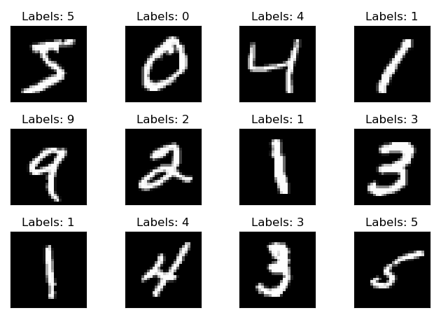
MNIST(Modified National Institute of Standards and Technology)是机器学习领域最著名的数据集之一,包含70,000张手写数字图像:
\[
\varphi = 1+\frac{1} {1+\frac{1} {1+\frac{1} {1+\cdots} } }
\]
训练集 :60,000张图像测试集 :10,000张图像图像尺寸 :28×28像素的灰度图类别数量 :10类(数字0-9)
regular
1.2 使用torchvision加载数据
1
2
3
4
5
6
7
8
9
from torchvision import datasets, transforms"./dataset" ,True ,True ,
关键参数说明 :
root:数据存储路径,会自动创建MNIST子目录train:True加载训练集,False加载测试集download:首次运行时自动从网络下载transform:数据转换操作,这里将PIL图像转为Tensor
数据存储结构 : 1 2 3 4 ./ dataset/ / / /
1.3 DataLoader:高效的数据加载器
1 2 3 4 5 6 7 8 from torch.utils.data import DataLoader64 ,True ,0
DataLoader的作用 :
批处理 (Batching):将样本组织成批次,提高GPU利用率打乱 (Shuffling):随机化训练顺序,避免模型记忆样本顺序并行加载 (Multi-processing):通过num_workers加速数据读取
最佳实践 : - 训练集:shuffle=True,打破样本相关性 - 测试集:shuffle=False,保持评估一致性 - batch_size:根据显存调整,常用32/64/128 - num_workers:Windows建议0,Linux/Mac可设为4-8
二、数据预处理与标准化
2.1 为什么需要数据预处理?
原始图像像素值范围是[0, 255],直接输入神经网络会导致:
梯度爆炸/消失 :数值过大导致梯度不稳定收敛缓慢 :不同特征量级差异大,优化困难激活函数饱和 :超出激活函数有效区间
2.2 标准化流程
1 2 3 4 transform = transforms.Compose([0.1307 ,), std=(0.3081 ,))
步骤1:ToTensor() - 将PIL图像/NumPy数组转为PyTorch张量 - 形状变换:[H, W, C] → [C, H, W] - 像素归一化:[0, 255] → [0, 1]
步骤2:Normalize() - 公式:output = (input - mean) / std - MNIST的全局统计值: - 均值(mean)= 0.1307 - 标准差(std)= 0.3081 - 结果:数据分布近似标准正态分布N(0, 1)
2.3 标准化的数学原理
对于每个像素值 \(x\) ,标准化操作为:
\[
x_{normalized} = \frac{x - \mu}{\sigma}
\]
其中 \(\mu\) 是均值,\(\sigma\) 是标准差。标准化后的数据具有: - 均值为0 - 标准差为1 - 消除量纲影响
为什么使用0.1307和0.3081?
这两个值是通过计算整个MNIST训练集的全局均值和标准差得到的:
1 2 3 255.0 255.0
三、CNN网络架构设计
3.1 卷积神经网络基础
卷积神经网络(CNN)是专门处理图像数据的深度学习架构,主要由以下组件构成:
卷积层 (Convolutional Layer):特征提取激活函数 (Activation):引入非线性池化层 (Pooling Layer):降维与特征选择全连接层 (Fully Connected Layer):分类决策
3.2 模型架构详解
1 2 3 4 5 6 7 8 9 10 11 12 13 14 15 16 17 18 19 20 21 22 23 24 class MNIST_CNN (nn.Module):def __init__ (self ):super (MNIST_CNN, self ).__init__()self .conv1 = nn.Sequential(1 , 10 , kernel_size=5 ),2 )self .conv2 = nn.Sequential(10 , 20 , kernel_size=5 ),2 )self .fc = nn.Sequential(320 , 50 ),50 , 10 )
3.3 特征图尺寸计算
输入层 :[batch_size, 1, 28, 28]
第一卷积模块 : - Conv2d(1→10, 5×5):[B, 1, 28, 28] → [B, 10, 24, 24] - 计算公式:\(H_{out} = H_{in} - kernel\_size + 1 = 28 - 5 + 1 = 24\) - MaxPool2d(2×2):[B, 10, 24, 24] → [B, 10, 12, 12] - 每个维度缩小一半:\(24 \div 2 = 12\)
第二卷积模块 : - Conv2d(10→20, 5×5):[B, 10, 12, 12] → [B, 20, 8, 8] - \(H_{out} = 12 - 5 + 1 = 8\) - MaxPool2d(2×2):[B, 20, 8, 8] → [B, 20, 4, 4] - \(8 \div 2 = 4\)
全连接层 : - Flatten:[B, 20, 4, 4] → [B, 320] - \(20 \times 4 \times 4 = 320\) - Linear(320→50):[B, 320] → [B, 50] - Linear(50→10):[B, 50] → [B, 10]
输出层 :[batch_size, 10],10个logits对应10个类别
3.4 关键层详解
卷积层(Conv2d)
1 nn.Conv2d(in_channels, out_channels, kernel_size)
作用 :通过卷积核滑动提取局部特征
参数 : - in_channels:输入通道数(灰度图=1,RGB=3) - out_channels:输出通道数(特征图数量) - kernel_size:卷积核大小(常用3×3, 5×5)
特点 : - 局部连接:只关注局部区域 - 权重共享:同一卷积核扫描整个图像 - 参数量:\(kernel\_size^2 \times in\_channels \times out\_channels\)
激活函数(ReLU)
公式 :\(ReLU(x) = max(0, x)\)
优点 : - 计算简单,训练速度快 - 缓解梯度消失问题 - 引入非线性,增强模型表达能力
池化层(MaxPool2d)
1 nn.MaxPool2d(kernel_size=2 )
作用 : - 降低特征图空间维度 - 减少参数量和计算量 - 提供平移不变性
MaxPooling vs AvgPooling : - MaxPooling:取区域最大值,保留显著特征 - AvgPooling:取区域平均值,保留整体信息
四、训练流程与优化策略
4.1 完整训练流程
1 2 3 4 5 6 7 8 9 10 11 12 13 14 15 16 17 18 19 20 21 22 def train (model, train_loader, optimizer, epoch ):for i in range (epoch):for batch_idx, data in enumerate (train_loader):0 ].to(device), data[1 ].to(device)
4.2 训练循环关键步骤
步骤1:数据加载
1 inputs, labels = data[0 ].to(device), data[1 ].to(device)
data是DataLoader返回的元组:(图像, 标签).to(device):将数据移动到GPU/CPU
步骤2:清零梯度
为什么需要?
PyTorch默认会累积梯度,如果不清零: 1 2 3 4 5
正确做法: 1 2 optimizer.zero_grad()
步骤3-4:前向传播与损失计算
1 2 outputs = model(inputs)
CrossEntropyLoss详解 :
\[
Loss = -\sum_{i=1}^{C} y_i \log(\hat{y}_i)
\]
其中: - \(y_i\) :真实标签的one-hot编码 - \(\hat{y}_i\) :经过softmax的预测概率
内部实现 : 1. 对logits应用softmax:\(\hat{y}_i = \frac{e^{z_i}}{\sum_{j=1}^{C} e^{z_j}}\) 2. 计算负对数似然损失
步骤5-6:反向传播与参数更新
1 2 loss.backward()
反向传播原理 :
通过链式法则计算损失对每个参数的偏导数:
\[
\frac{\partial L}{\partial w} = \frac{\partial L}{\partial y} \cdot \frac{\partial y}{\partial w}
\]
参数更新(SGD) :
\[
w_{new} = w_{old} - \eta \cdot \frac{\partial L}{\partial w}
\]
其中 \(\eta\) 是学习率(learning rate)
4.3 优化器选择
1 2 3 4 5 optimizer = optim.SGD(0.01 ,0.9
SGD with Momentum
标准SGD : \[
w_{t+1} = w_t - \eta \cdot g_t
\]
带动量的SGD : \[
v_{t+1} = \beta \cdot v_t + g_t
\] \[
w_{t+1} = w_t - \eta \cdot v_{t+1}
\]
优点 : - 加速收敛:借助历史梯度的“惯性” - 减少震荡:平滑梯度更新方向 - 跳出局部最优:动量帮助越过小的“山谷”
其他常用优化器
SGD
简单稳定
计算机视觉任务
Adam
自适应学习率
大多数深度学习任务
AdamW
Adam + 权重衰减
Transformer模型
RMSprop
自适应学习率
RNN任务
4.4 学习率调度
固定学习率可能导致: - 初期:学习率过小,收敛慢 - 后期:学习率过大,无法收敛
常用策略 :
1 2 3 4 5 6 7 8 30 , gamma=0.1 )100 )10 )
五、模型评估与可视化
5.1 评估指标体系
准确率(Accuracy)
\[
Accuracy = \frac{正确预测数}{总样本数}
\]
优点 :直观易懂 缺点 :类别不平衡时会误导
精确率(Precision)
\[
Precision = \frac{TP}{TP + FP}
\]
含义 :预测为正例中,真正为正例的比例
召回率(Recall)
\[
Recall = \frac{TP}{TP + FN}
\]
含义 :真实正例中,被正确预测的比例
F1分数
\[
F1 = 2 \cdot \frac{Precision \times Recall}{Precision + Recall}
\]
含义 :精确率和召回率的调和平均
5.2 使用sklearn生成分类报告
1 2 3 4 5 6 7 8 9 10 11 12 13 14 15 from sklearn.metrics import classification_reporteval ()with torch.no_grad():for x, y in test_loader:1 ).cpu()print (classification_report(y_trues, y_preds, target_names=classes))
输出示例 : 1 2 3 4 5 6 7 8 9 precision recall f1-score support0 0.98 0.99 0.99 980 1 0.99 0.99 0.99 1135 2 0.98 0.97 0.98 1032 0.98 10000 macro avg 0.98 0.98 0.98 10000 0.98 0.98 0.98 10000
5.3 混淆矩阵可视化
1 2 3 4 5 6 7 8 9 10 from sklearn.metrics import confusion_matrix, ConfusionMatrixDisplay"Confusion Matrix" )
混淆矩阵解读 :
1 2 3 4 5 6 预测 0 1 2 ... 0 [950 0 2 ...] 1 [ 0 980 1 ...] 2 [ 3 1 970 ...]
对角线:正确预测数量
非对角线:误分类情况
行和:每个类别的真实数量
列和:每个类别的预测数量
常见误分类分析 : - 数字1和7容易混淆 - 数字4和9容易混淆 - 数字3和8容易混淆
5.4 模型预测流程
1 2 3 4 model.eval () with torch.no_grad(): 1 )
为什么需要model.eval()?
训练模式和评估模式的区别:
Dropout
随机丢弃神经元
保留所有神经元
BatchNorm
使用批次统计
使用全局统计
梯度计算
开启
关闭(配合no_grad)
六、常见问题与优化建议
6.1 代码中的潜在问题
问题1:全连接层缺少激活函数
1 2 3 4 5 6 7 8 9 10 11 12 13 14 15 self .fc = nn.Sequential(320 , 50 ),50 , 10 ) self .fc = nn.Sequential(320 , 50 ),0.5 ), 50 , 10 )
问题2:未创建checkpoints目录
1 2 3 import os'./checkpoints' , exist_ok=True )
问题3:固定学习率
1 2 3 4 5 6 7 30 , gamma=0.1 )for epoch in range (100 ):
6.2 性能优化策略
1. 数据增强
1 2 3 4 5 6 transform_train = transforms.Compose([10 ), 0 , translate=(0.1 , 0.1 )), 0.1307 ,), (0.3081 ,))
效果 :增加训练样本多样性,提升泛化能力
2. 批标准化(Batch Normalization)
1 2 3 4 5 6 self .conv1 = nn.Sequential(1 , 10 , kernel_size=5 ),10 ), 2 )
优点 : - 加速训练 - 允许更大学习率 - 减少对初始化的依赖
3. 残差连接(ResNet思想)
1 2 3 4 5 6 7 8 9 10 11 12 13 class ResBlock (nn.Module):def __init__ (self, channels ):super ().__init__()self .conv = nn.Sequential(3 , padding=1 ),3 , padding=1 ),def forward (self, x ):return F.relu(self .conv(x) + x)
4. 混合精度训练
1 2 3 4 5 6 7 8 9 10 11 12 13 14 from torch.cuda.amp import autocast, GradScalerfor data in train_loader:with autocast():
效果 :显存占用减少50%,训练速度提升2-3倍
6.3 超参数调优建议
学习率
1e-4 ~ 1e-1
网格搜索/学习率查找器
batch_size
32 ~ 256
根据显存调整
卷积核大小
3×3, 5×5
小卷积核更常用
Dropout率
0.3 ~ 0.5
防止过拟合
6.4 调试技巧
检查数据维度
1 2 3 print (f"Input shape: {inputs.shape} " )print (f"Output shape: {outputs.shape} " )print (f"Label shape: {labels.shape} " )
可视化特征图
1 2 3 4 5 6 7 8 9 10 11 12 13 14 15 16 17 18 19 20 def visualize_feature_maps (model, image ):def hook (name ):def fn (module, input , output ):return fn'conv1' ))with torch.no_grad():'conv1' ].squeeze()2 , 5 , figsize=(12 , 5 ))for i, ax in enumerate (axes.flat):'viridis' )'off' )
梯度检查
1 2 3 4 for name, param in model.named_parameters():if param.grad is not None :print (f"{name} : grad_norm = {param.grad.norm():.4 f} " )
七、进阶扩展
7.1 模型压缩
1 2 3 4 5 6 7 8 9 10 1 ),1 ),'batchmean'
7.2 迁移学习
1 2 3 4 5 6 7 8 9 'mnist_best.pth' )for param in model.conv1.parameters():False 0.001 )
7.3 模型集成
1 2 3 4 5 6 7 8 9 10 11 12 for model in models:eval ()with torch.no_grad():1 )0 )[0 ]
八、总结
本文详细介绍了使用PyTorch构建MNIST手写数字识别系统的完整流程,涵盖了:
核心技术点 : - 数据加载与预处理 - CNN网络架构设计 - 训练流程与优化 - 模型评估与可视化
关键要点 : 1. 数据标准化是提升模型性能的基础 2. CNN通过卷积和池化提取图像特征 3. 合理的优化器和学习率调度至关重要 4. 多维度评估指标全面了解模型性能
优化方向 : - 数据增强提升泛化能力 - Batch Normalization加速训练 - Dropout防止过拟合 - 混合精度训练提升效率
实践建议 : - 从简单模型开始,逐步增加复杂度 - 重视数据质量和预处理 - 定期保存模型和可视化训练过程 - 使用TensorBoard监控训练指标
参考资源
官方文档
进阶阅读
代码仓库
附录:完整代码清单
A. 改进版模型
1 2 3 4 5 6 7 8 9 10 11 12 13 14 15 16 17 18 19 20 21 22 23 24 25 26 27 28 29 30 31 32 33 34 35 36 37 38 39 40 class ImprovedMNIST_CNN (nn.Module):def __init__ (self ):super (ImprovedMNIST_CNN, self ).__init__()self .conv1 = nn.Sequential(1 , 32 , kernel_size=3 , padding=1 ),32 ),32 , 32 , kernel_size=3 , padding=1 ),32 ),2 , 2 ),0.25 )self .conv2 = nn.Sequential(32 , 64 , kernel_size=3 , padding=1 ),64 ),64 , 64 , kernel_size=3 , padding=1 ),64 ),2 , 2 ),0.25 )self .fc = nn.Sequential(64 * 7 * 7 , 256 ),256 ),0.5 ),256 , 10 )def forward (self, x ):self .conv1(x)self .conv2(x)self .fc(x)return x
B. 完整训练脚本
1 2 3 4 5 6 7 8 9 10 11 12 13 14 15 16 17 18 19 20 21 22 23 24 25 26 27 28 29 30 31 32 33 34 35 36 37 38 39 40 41 42 43 44 45 46 47 48 49 50 51 52 53 54 55 56 57 58 59 60 61 62 63 64 65 66 67 68 69 def train_improved (model, train_loader, val_loader, epochs=50 ):'cuda' if torch.cuda.is_available() else 'cpu' )0.001 )'min' , patience=5 , factor=0.5 0.0 'train_loss' : [], 'val_loss' : [], 'val_acc' : []}for epoch in range (epochs):0.0 for inputs, labels in train_loader:eval ()0.0 0 0 with torch.no_grad():for inputs, labels in val_loader:max (1 )0 )sum ().item()len (train_loader)len (val_loader)100. * correct / total'train_loss' ].append(train_loss)'val_loss' ].append(val_loss)'val_acc' ].append(val_acc)print (f'Epoch {epoch+1 } /{epochs} :' )print (f' Train Loss: {train_loss:.4 f} ' )print (f' Val Loss: {val_loss:.4 f} , Val Acc: {val_acc:.2 f} %' )if val_acc > best_acc:'best_model.pth' )print (f' Best model saved! (Acc: {best_acc:.2 f} %)' )return history
C. 可视化工具
1 2 3 4 5 6 7 8 9 10 11 12 13 14 15 16 17 18 19 20 21 22 def plot_training_history (history ):1 , 2 , figsize=(12 , 4 ))'train_loss' ], label='Train Loss' )'val_loss' ], label='Val Loss' )'Epoch' )'Loss' )'Training and Validation Loss' )True )'val_acc' ], label='Val Accuracy' , color='green' )'Epoch' )'Accuracy (%)' )'Validation Accuracy' )True )
作者 :[您的名字]日期 :2024年版本 :1.0
本文所有代码均已在PyTorch 2.0+环境下测试通过。如有问题欢迎交流讨论!